
optimal (LQ) control algebraic riccati equations \(\small \dot{\textbf{P}}=-\textbf{P}(t)\textbf{A}(t)-\textbf{A}^T(t)\textbf{P}(t)+\textbf{P}(t)\textbf{B}(t)\textbf{R}^{-1}(t)\textbf{B}^T(t)\textbf{P}(t)-\textbf{Q}(t) \) with Hamilton approach \(\small \mathcal{H} = \parallel \underline{x}(t)\parallel^2_{\textbf{Q}(t)} +\parallel\underline{u}(t)\parallel^2_{\textbf{R}(t)} + \underline{\lambda}^T \left(\textbf{A}(t)\underline{x} +\textbf{B}(t)\underline{u}(t)\right).\)
nonlinear control; flatness-based control linear system dynamics \(\tiny y^{(n)}-y_{ref}^{(n)}-a_{n-1}\left( y_{ref}^{(n-1)} - y^{(n-1)}\right)-\ldots -a_{1}\left(\dot{y}_{ref}-\dot{y} \right) -a_0(y_{ref}-y) \stackrel{!}{=} 0 \) flatness controller: \(\small u(t) = \Psi_2\left( y(t), \dot{y},\ldots, y^{(n-1)}, y^{n} \right) .\)
- Sliding control Assume, that exists; a nonlinear (single-input affine) system \(\underline{x}^{(n)}= f(\underline{x})+b(\underline{x})u\); sliding condition \(\frac{1}{2}\frac{d}{dt} s^2 \le -\eta |s|\); the tracking error vector is \(\underline{\tilde{x}} = \underline{x}-\underline{x}_{desired}\); furthermore, let us define a time-varying surface S(t) in the state-space \(R^{(n)}\) by the scalar equation \(s(\underline{x};t) = 0\) , where \(s(\underline{x};t)=\left( \frac{1}{dt} +\lambda\right)^{n-1} \underline{\tilde{x}}\) and \(\lambda\) is a strictly positive constant. For instance, if n=2, the following equation applies \(s = \underline{\dot{\tilde{x}}}+\lambda \underline{\tilde{x}}\) . For example \(\ddot{x} = f(x) +u \) where \(u\) is the control input, \(x\) is the output of interest, and the dynamics \(f\) is not exactly known, but estimated as \(\hat{f}\). The estimation error on \(f\) is assumed to be bounded by some known function \(F = F(x,\dot{x}) ~~~ |f-\hat{f}| \le F\). The control input is \(u = \hat{u}-(F+\eta)\cdot sign(s) ~~with~~ \hat{u}= -\hat{f}+\ddot{x}_{desired}- \lambda \dot{\tilde{x}}\) .
- Slotine, J.-J. E. and Li, W.: Applied Nonlinear Control. Prentice Hall, Englewood Cliffs, N.J, 1st edition, 1991. p.276f.
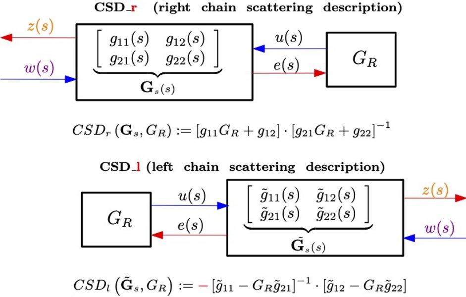
chain scattering-matrix description (CSD)
- chain scattering-matrix description (CSD) of a two-port network
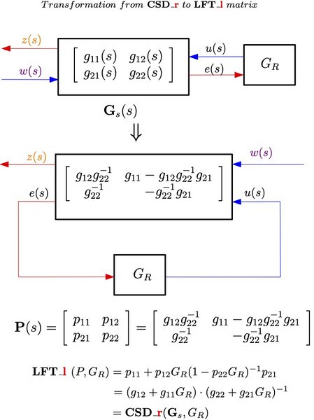
- linear (lower) fractional transformation \(\small \underbrace{\left(\textbf{P}_{11} +\textbf{P}_{12} \textbf{G}_R \left( \textbf{I}-\textbf{P}_{22} \textbf{G}_R\right)^{-1}\textbf{P}_{21}\right)}_{\mathcal{F}_l({\textbf{P}},\textbf{G}_R)} \underline{w} \)
- coprime factorization
- \(\small G(s) = N(s)M^{-1}(s)=\tilde{M}(s)\tilde{N}^{-1}(s) ~with \\ \small numerator~and ~denominator ~matrices~ of ~right-~sided ~and\\ \small left-sided ~ coprime~ factorizations\\ \small \left[\begin{array}{c} N(s) \\ M(s) \end{array}\right] \stackrel{}{=} \begin{bmatrix} \begin{array}{c|c} A+BF & BW \\ \hline C+DF & DW \\ F & W \end{array} \end{bmatrix}\\ \small\left[\begin{array}{cc} \tilde{N}(s) & \tilde{M}(s) \end{array}\right] \stackrel{}{=} \begin{bmatrix} \begin{array}{c|cc} A+HC & B+HD & H \\ \hline \tilde{W}C & \tilde{W}D & \tilde{W} \end{array} \end{bmatrix} \\ \small \textbf{Bezout-Identity}\\ \tiny (Raisch, J.: Mehrgrößenregelung~ im ~Frequenzbereich, Oldenbuorg~ Verlag, 1994.p.84f.) \\ \small \left[ \begin{array}{cc} X(s) & Y(s) \\ \tilde{M}(s) & -\tilde{N} (s) \end{array} \right] \cdot \left[ \begin{array}{cc} N(s) & \tilde{Y}(s) \\ M(s) & -\tilde{X}(s) \end{array} \right] = \left[ \begin{array}{cc} \textbf{I}_r & \textbf{0} \\ \textbf{0} & \textbf{I}_m \end{array} \right] \)
- normalized (right) coprime factorization\(\small P(s) =\left[\begin{array}{c} M(s) \\ N(s) \end{array}\right] \stackrel{}{=} \begin{bmatrix} \begin{array}{c|c} A+BF & BW \\ \hline F & W\\ C+DF & DW \end{array} \end{bmatrix}\\ \small P^{\tilde ~}(s)=P^T(-s) ~\checkmark\\ \small P^{\tilde~}(s)\cdot P(s) = \left[\begin{array}{cc} M^{\tilde~} & N^{\tilde~} \end{array}\right]\cdot \left[\begin{array}{c} M \\ N \end{array}\right]= \textbf{I}\\ \small P^{\tilde~}(s)=\left[\begin{array}{cc} M^{\tilde~} & N^{\tilde~} \end{array}\right]\stackrel{s}{=} \begin{bmatrix} \begin{array}{c|cc} -(A+BF) & F^T & (C+DF)^T \\ \hline -W^TB^T & W^T & W^TD^T \end{array} \end{bmatrix}\\ \small \textbf{Note}; M^{\tilde~}\ne \tilde{M} ~and~ N^{\tilde~}\ne \tilde{N}\)
- example (normalized (right) coprime factorization); unstable (linear) system \(\small \underline{\dot{x}} = \left[\begin{array}{*{2}{c}} 3 & -2\\ 1 & 0 \end{array} \right]\underline{x}+ \left[\begin{array}{*{1}{c}} 1 \\ 0 \end{array} \right]u\\ \small y= \left[\begin{array}{*{2}{c}} -2 & -10 \end{array} \right]\underline{x} -2u\\ \small G_s(s)=\frac{2(s^2-4s+3)}{(s-1)((s-2)}\)
- \(\small u_{pole} = \left[\begin{array}{*{2}{c}} 4.6000 & -1.1100 \end{array} \right]\underline{x} -0.1483w ~\checkmark\\ \small u_{schur} = \left[\begin{array}{*{2}{c}} 0.0233 & 0.0349 \end{array} \right]\underline{x} -0.3275w ~\checkmark\\ \small u_{riccati} = \left[\begin{array}{*{2}{c}} -14.3923 & -8.3923 \end{array} \right]\underline{x} -1.7321w ~\checkmark\)
- Tsai, Min-Ching and Gu, Da-Wei: Robust and Optimal Control; A Two-port Framework Approach. 1st Edition, Springer Verlag London, 2014.