Exact linearization with internal dynamics

• For non-linear systems, linearization can be performed at the operating point (Taylor linearization). A linear system is obtained, which (however) only has validity in a small vicinity of the operating point. 
• The Harmonic Balance method is mainly used for   system analysis. With this method  important system properties, such as the continuous oscillations, can be determined,  which can be interpreted for a stable behavior of the non-linear control loop. 
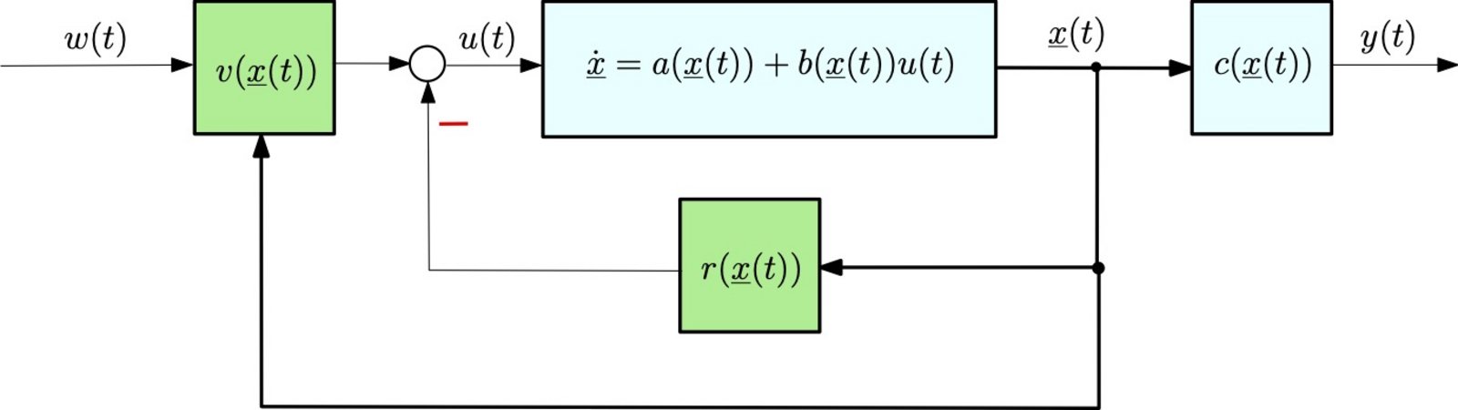
• We will now describe a method which enables us to design controllers for nonlinear plants directly, not utilizing a linear approximation of the non- linear plant. The basic concept is to design a nonlinear controller so that it completely compensates for the nonlinearity of the plant, thereby creating a linear control loop.

Given a non-linear (input-affine) system

\(\dot{\underline{x}} = a(\underline{x}(t)) + {b}(\underline{x}(t)) \cdot u(t) , \quad y(t)= {c}(\underline{x}(t)).\)

The non-linear system is converted exactly into a linear system by means of a non-linear coordinate transformation and a non-linear feedback law -> Input-Output Linearization.

We start by calculating the time derivative of the output variable y and obtain

\(\dot{y}= \left[\frac{\partial c(\underline{x}(t))}{\partial x_1} \ldots \frac{\partial c(\underline{x}(t))}{\partial x_n}\right]^T \cdot \left[\begin{array}{c} \dot{x}_1\\ \vdots \\ \dot{x}_n\\ \end{array} \right] = \left[ \frac{dc(\underline{x}(t))}{d\underline{x}} \right]^T\dot{\underline{x}} = \frac{\partial c(\underline{x})}{\partial\underline{x}}\dot{\underline{x}}\)

Substituting into the equation \(\dot{\underline{x}}(t) =        a(\underline{x}(t)) + {b}(\underline{x}(t))u(t)  \) yields

\(\dot{y} = \underbrace{\frac{\partial c(\underline{x})}{\partial\underline{x}}a(\underline{x}(t))}_{L_a c(\underline{x}(t))} + \underbrace{\frac{\partial c(\underline{x})}{\partial\underline{x}}{b}(\underline{x}(t))}_{L_b c(\underline{x}(t))} \cdot u(t). \)
For most technical systems, in the above equation \(L_b c(\underline{x}(t))=0\) holds so that we obtain

\(\dot{y} = L_a c(\underline{x}(t)) \)

Next, the second time derivative \(\ddot{y}\)  is to be determined. Starting with \(\dot{y} =  L_a c(\underline{x}(t))\), we obtain the 
expression

\(\ddot{y} = \underbrace{\frac{\partial L_a c(\underline{x}(t))}{\partial\underline{x}} a(\underline{x}(t))}_{L_aL_ac(\underline{x})} + \underbrace{\frac{\partial L_a c(\underline{x}(t))}{\partial \underline{x}} {b}(\underline{x}(t))}_{L_bL_ac(\underline{x})} \cdot u(t)\)

We refer to \(\delta\)  as the difference degree or mostly as the relative degree of the system. For linear systems, the relative degree is equal to the difference  between the denominator degree n and the numerator degree m of the transfer function, that means \(\delta=n-m\). In this sequence of time derivatives, the equation 

\( L_bL_a^ic(\underline{x}(t))=\frac{\partial L_a^i c(\underline{x}(t))}{\partial \underline{x}}{b}(\underline{x}(t))= 0.\)

holds for all indices  \(i=1,2,\ldots, \delta-2\). The Lie derivative \(L_bL_a^ic(\underline{x}(t))\) is not equal to zero only for indices \(i \ge  \delta-1\). We refer to \(\delta\) as the difference degree or mostly as the relative degree of the system. The relative degree indicates the
degree of the output variable y derivative at which it directly depends on the control variable 
 u for the first time; that means, for \(i=\delta-1\)  holds \(         \frac{\partial L_a^{i=\delta-1} c(\underline{x}(t))}{\partial         \underline{x}}{b}(\underline{x}(t))\neq 0\).

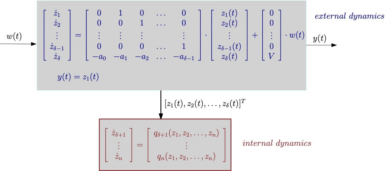
Internal Dynamics

In this chapter, the case \(\delta < n\) is considered; this is the case when the \textbf{relative degree} \(\delta\) is reduced compared to the system order n. In this case, too, a nonlinear transformation, here a diffeomorphism \(\underline{z}=\underline{\eta}(\underline{x})\), a system representation favorable for the controller design  system representation can be found. 

Since \( \delta<n\)  holds,only the first \(\delta\)  components \(\eta_1, \ldots, \eta_\delta\) of the diffeomorphism \(\underline{z}=\underline{\eta}(\underline{x})\) can be used for the new state variables \( z_1,\ldots, z_n\) in the same form as in the case in which \(\delta = n\) holds. It holds that 

\(\underline{z}(t)= \left[ \begin{array}{c} \\[-0.5cm] z_1(t)\\ z_2(t)\\ z_3(t)\\ \vdots \\ z_{\delta}(t)\\ z_{\delta+1}(t)\\ \vdots \\ z_n(t) \end{array} \right] = \left[ \begin{array}{} \\[0.1cm] c(\underline{x}(t))\\ L_a c(\underline{x}(t))\\ L^2_a c(\underline{x}(t))\\ \vdots \\ L^{\delta-1}_a c(\underline{x}(t))\\ \eta_{\delta+1}(\underline{x}(t))\\ \vdots \\ \eta_n(\underline{x}) \end{array} \right] =\underline{\eta}(\underline{x}(t)). \)

Using the transformation \(\underline{x}(t)= \underline{\eta}^{-1}(\underline{z}t))\) the (temporal) derivation

\(\dot{\eta}_i(\underline{x}(t))= \frac{\partial \eta_i(\underline{x})}{\partial \underline{x}}\cdot \dot{\underline{x}} = \frac{\partial \eta_i(\underline{x})}{\partial \underline{x}}\left[ a(\underline{x})+\underline{b}(\underline{x})\cdot u \right]\)

\(\dot{\eta}_i(\underline{x})=L_a\eta_i(\underline{x})+L_b\eta_i(\underline{x})\cdot u = \hat{q}_i(\underline{x}, u)= q_i(\underline{z},u)\)

If the function \( \eta_i\) is chosen so that
\( L_b\eta_i(\underline{x}) = \frac{\partial \eta_i(\underline{x})}{\partial \underline{x}}\underline{b}(\underline{x}) = 0 \)

then above Equation is simplified. Because now the dependence on the input variable u, and the following holds
\(\dot{\eta}_i = L_a\eta_i(\underline{x})=\hat{q}_i(\underline{x})=q_i(\underline{z}).\)

However, the eq. \( L_b\eta_i(\underline{x}) = \frac{\partial \eta_i(\underline{x})}{\partial \underline{x}}\underline{b}(\underline{x}) = 0 \) is a partial differential equation, which can lead to problems when solving it. 

• _{Adamy J.: Nonlinear systems and controls. Springer-Verlag, 1th edition, 2022 (corrected publication 2023).} \(\checkmark\)
• _{Föllinger, O.: Nichtlineare Regelungen, Bd. 2: Harmonische Balance, Popow- und Kreiskriterium. Oldenbourg Verlag München, 7. Auflage, 1993.} \(\checkmark\)
• _{Khalil, H. K: Nonlinear Systems. Prentice Hall, Upper Saddle River, N.J., 3rd edition, 2002.} \(\checkmark\) 
• _{Slotine, J.-J. E. and Li, W.: Applied Nonlinear Control. Prentice Hall, Englewood Cliffs, N.J, 1st edition, 1991.} \(\checkmark\)

_{\(\checkmark~~books ~recommendable\)}